Using the standalone classes and functions
Different histograms can be computed using the available standalone classes jackHI provides in the hogg_jackknife module. Visualization can also be performed using the hi_plot module.
Note
I give examples for count histograms. Probability and probability density histograms can straightforwardly be obtained using similar procedures, by altering the input objects slightly.
Count histogram
Non-optimized histograms
Here, I show how to use jackHI to create simple histograms based on the user input objects.
Constant width
To make a simple histogram that displays the counts per bin, one can execute:
from hogg_jackknife import UserBools, UserInput, Hist
import numpy as np

# set up the input objects
my_bools = UserBools()
my_input = UserInput(
    data_arr=np.array([0.25, 1.25, 2.50, 4.00]),
    min_nr_bins=0,
)

# initialize the 'Hist' object
my_hist = Hist(user_bools=my_bools, user_input=my_input)

# compute the histogram for a constant bin width
my_hist.specific_width(
    bin_phase=0.0, # no binning phase
    bin_nr=10, # use 10 bins
    data_min=None, # set the data minimum to the minimum of the supplied data array
    bin_width=None, # automatically calculate the bin width
)
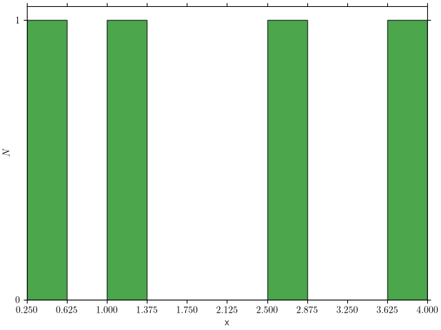
This Hist object should then contain the histogram data.
In particular, the attribute hist_data should be equal to [1.0, 0.0, 1.0, 0.0, 0.0, 1.0, 0.0, 0.0, 1.0, 0.0].
The histogram contained within this Hist object can be visualized using the functionalities and input classes defined in the hi_plot module:
from hi_plot import HistogramPlotSave, HistogramPlotSetup, plot_histogram

# set up the input objects
hsave = HistogramPlotSave() # default saving options
hsetup = HistogramPlotSetup(
    x_label="x",
    label_kwargs=None,
    figure_kwargs={"constrained_layout": True},
    plot_kwargs=None,
    use_latex=True
)

# plot the histogram
plot_histogram(
    histogram_object=my_hist, # this is the histogram object in which computed data are stored
    setup_args=hsetup,
    save_args=hsave,
    display_plot=True,
)
Issuing these commands should result in a plot that looks like this:
Logarithmic width
The procedure to generate a logarithmic-width histogram is very similar. The following commands should be issued to compute it:
from hogg_jackknife import UserBools, UserInput, Hist
import numpy as np

# set up the input objects
my_bools = UserBools()
my_input = UserInput(
    data_arr=np.array([0.01, 0.5, 0.2, 2.00, 20.0, 200.0]), # more appropriate data for log binning
    min_nr_bins=0,
)

# initialize the 'Hist' object
my_hist = Hist(user_bools=my_bools, user_input=my_input)

# compute the histogram for a logarithmic bin width
my_hist.logarithmic_width(
    bin_edges=np.logspace(-2,3,num=6), # from 0.01 to 1000.0
)
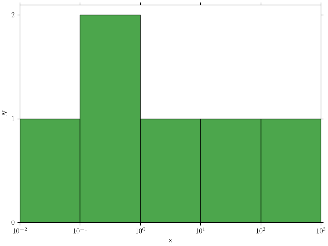
This Hist object should then contain the logarithmically binned histogram data.
In particular, its attribute hist_data should be equal to [1.0, 2.0, 1.0, 1.0, 1.0].
The commands to visualize it using hi_plot are exactly the same as before (and will therefore not be repeated). They should result in a plot that looks like this:
Optimized histograms
Here, I show how to use jackHI's built-in optimization procedures to perform data-based bin width selection and generate the optimal histograms.
Constant width
A more interesting example maximizes the jackknife likelihood of a small data array:
from hogg_jackknife import (
    UserBools,
    UserHoggBools,
    UserHoggInput,
    JackHist,
)
import numpy as np

# set up the input objects
my_bools = UserBools()
hogg_bools = UserHoggBools(
    verbose=False,
    return_binning_parameters=True,
)
hogg_input = UserHoggInput(
    data_arr=np.array([0.0, 1.0, 2.0, 3.0, 10.0, 10.5, 11.0, 19.0, 18.0, 20.0, 28.0, 36.0, 42.0, 50.0, 45.0]),
    alpha_parameters=np.array([0.2, 1.0, 2.0]), # set alpha smoothing parameters
    bin_numbers=np.arange(1, 10, 1), # set a variety of bin numbers
    bin_phases=np.linspace(0.0, 0.3, num=31, endpoint=True), # set a variety of binning phases
    custom_bin_width=None,
)

# initialize the JackHist object
my_jack_hist = JackHist(
    user_bools=my_bools,
    user_input=hogg_input,
    hogg_bools=hogg_bools,
)

# compute the histogram
my_jack_hist.specific_width()
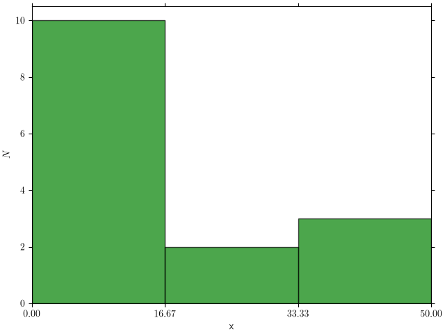
The expected optimized values are:
histogram_counts = np.array( # my_jack_hist.hist_data
    [10.0, 2.0, 3.0],
)
histogram_edges = np.array( # my_jack_hist.hist_edges
    [0.0, 50.0/3.0, 100.0/3.0, 50.0],
)
bin_width = np.array( # my_jack_hist.hist_width
    [50.0/3.0],
)
nr_bins = 3 # my_jack_hist.nr_bins
bin_phase = 0.21 # my_jack_hist.bin_phase
bin_alpha = 2.0 # my_jack_hist.bin_alpha
logarithmic_computation = False # my_jack_hist.logarithmic_computation
which are stored in the attributes of the JackHist object listed in the Pythonic comments above.
Visualization using hi_plot can again be done using the commands listed above, which result in the following plot:
Logarithmic width
This example maximizes the jackknife likelihood of a small data array in log-space:
from hogg_jackknife import (
    UserBools,
    UserHoggBools,
    UserHoggInput,
    JackHist,
)

# set up the input objects
hogg_input = UserHoggInput(
    data_arr=np.array([0.01, 0.2, 2.00, 20.0, 100.0]),
    alpha_parameters=np.array([0.2, 1.0, 2.0]),
    bin_numbers=np.array([1, 2, 4]),
    bin_phases=np.array([0.25, 0.5, 0.75]),
    custom_bin_width=None,
)
my_bools = UserBools()
hogg_bools = UserHoggBools(
    verbose=False,
    return_binning_parameters=True,
)

# initialize the JackHist object
my_jack_hist = JackHist(
    user_bools=my_bools,
    user_input=hogg_input,
    hogg_bools=hogg_bools,
)

# compute the histogram
my_jack_hist.logarithmic_width()
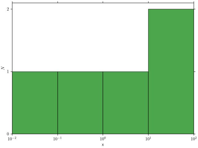
The expected optimized values are:
histogram_counts = np.array( # my_jack_hist.hist_data
    [1.0, 1.0, 1.0, 2.0],
)
histogram_edges = np.array( # my_jack_hist.hist_edges
    [0.01, 0.1, 1.0, 10.0, 100.0],
)
bin_widths = np.array( # my_jack_hist.hist_width
    [0.09, 0.9, 9.0, 90.0],
)
nr_bins = 4 # my_jack_hist.nr_bins
bin_phase = 0.25 # my_jack_hist.bin_phase
bin_alpha = 2.0 # my_jack_hist.bin_alpha
logarithmic_computation = True # my_jack_hist.logarithmic_computation
which are stored in the attributes of the JackHist object listed in the Pythonic comments above.
Visualization using hi_plot can again be done using the commands listed above, which result in the following plot: